Introduction to the espm
This tutorial will show you the basic operations of the toolbox. After installing the package with pip, start by opening a python shell, e.g. a Jupyter notebook, and import espm. The package espm is built on top of the hyperspy and the scikit-learn packages.
The hyperspy package is a Python library for multidimensional data analysis. It provides the base framework to handles our data. The scikit-learn package is a Python library for machine learning. It provides the base framework to for the Non Negative Matrix Factorization (NMF) algorithms develeoped in this package.
>>> import numpy as np
>>> import matplotlib.pyplot as plt
>>> import hyperspy.api as hs
>>> import espm
Datasets
Let us start by creating some data to play with this tutorial. We can generating artificial datasets using the following lines:
>>> import espm.datasets as ds
>>> ds.generate_built_in_datasets(seeds_range=1)
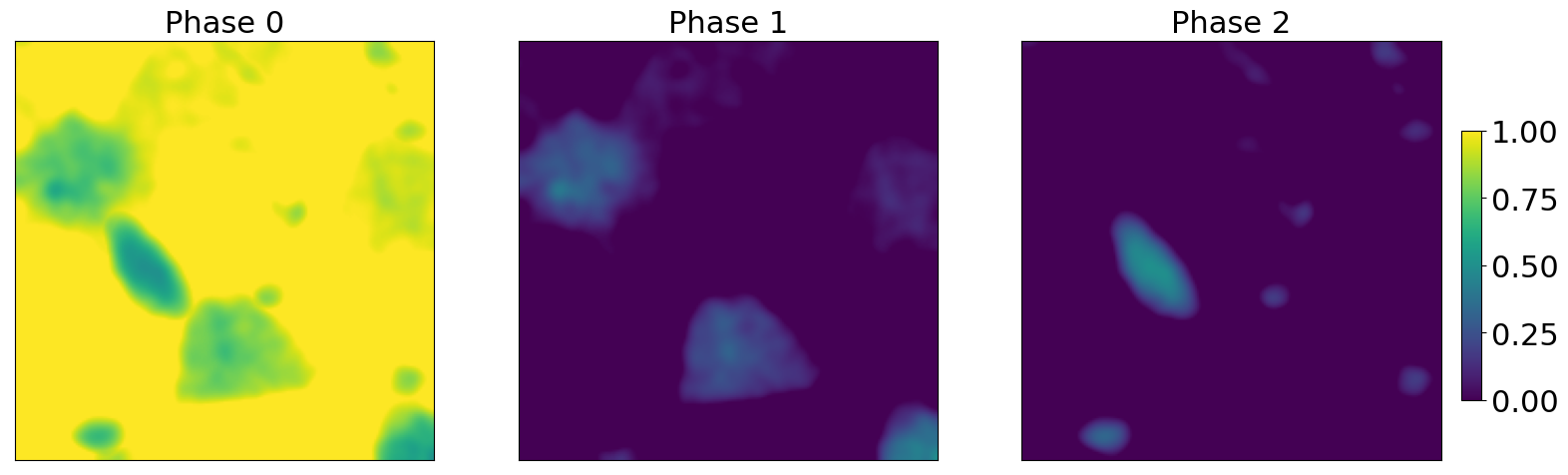
>>> spim = ds.load_particules(sample = 0)
>>> spim.change_dtype('float64')
The command generate_built_in_datasets will save the generated datasets folder defined in the espm.conf.py file. Alternatively, you can also define the path where the data will be saved using the “base_path” argument.
>>> ds.generate_built_in_datasets(base_path="generated_samples", seeds_range=1)
Here the object spim is of the espm.datasets.eds_spim.EDS_spim.
It inheritates from the hyperspy.api.signals.Signal1D class for a seamless integration in the hyperspy framework.
This object also has additional attributes and methods to store simulated ground truth and get the results of the decomposition performed using the espm package.
Note
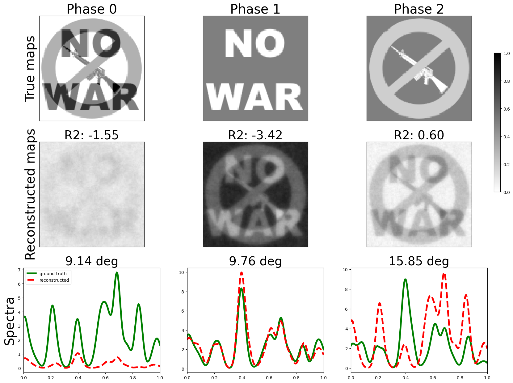
Please see the review article espm : a Python library for the simulation of STEM-EDXS datasets for an overview of the simulation methods this package leverages.
Including physics modelling in the decomposition
To improve the hyperspectral unmixing of the data, espm offers the opportunity to include physics modelling in the decomposition throught the G matrix.
The G matrix is easily built using the metadata store in the spim object.
>>> spim.build_G()
The G matrix is stored in the spim object and can be accessed using the G attribute.
The first columns of G correspond to the characteristic X-rays of the chemical elements that compose the sample and the two last columns correspond to the bremsstrahlung model.
The modelling of the characteristic X-rays is based on tables produced using the emtables package.
Factorization
Using the espm.estimators.SmoothNMF, we can use the physics-guided NMF algorithm to decompose the data.
The syntax of the hyperspy package can be used for the decomposition and plotting of the results.
>>> from espm.estimators import SmoothNMF
>>> est = SmoothNMF( n_components = 3, max_iter = 500, G = spim.G,hspy_comp = True,l2 = True,lambda_L = 0)
>>> out = spim.decomposition(True,algorithm= est)
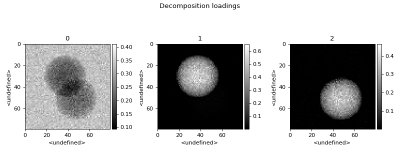
>>> spim.plot_decomposition_loadings(3)
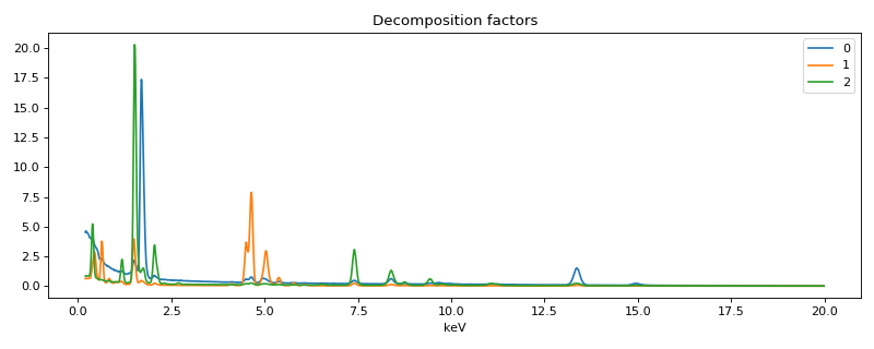
>>> spim.plot_decomposition_factors(3)
Thanks to the physics-guided approach a direct quantification is possible.
>>> spim.print_concentration_report()
Concentrations report
+----------+-----------+-------------+-----------+------------+-----------+-------------+
| Elements | p0 (at.%) |  p0 std (%) | p1 (at.%) | p1 std (%) | p2 (at.%) |  p2 std (%) |
+----------+-----------+-------------+-----------+------------+-----------+-------------+
| V        |     4.277 |       0.815 |     0.345 |      5.236 |     0.000 |    5426.331 |
| Rb       |    89.219 |       0.150 |     0.000 |   1217.568 |     0.000 |   10598.096 |
| W        |     6.505 |       0.430 |     0.000 | 329274.377 |     0.000 |      93.434 |
| N        |     0.000 | 3363320.886 |    52.263 |      0.848 |     0.000 |     423.423 |
| Yb       |     0.000 | 1047375.510 |    38.941 |      0.306 |     0.000 | 1344821.409 |
| Pt       |     0.000 | 1056115.710 |     8.450 |      0.663 |     0.000 |     172.134 |
| Al       |     0.000 | 2353678.504 |     0.000 |    307.917 |    23.854 |       0.781 |
| Ti       |     0.000 | 1773459.648 |     0.000 |    447.319 |    23.390 |       0.594 |
| La       |     0.000 | 1510548.956 |     0.000 |  15734.933 |    52.756 |       0.337 |
+----------+-----------+-------------+-----------+------------+-----------+-------------+
It uses algorithms that will be presented in a coming contribution.
These algorithms are an important part of this package. They are specialized to solve regularized Poisson NMF problems. Mathematically, they can be expressed as:
Here \(D_{GKL}\) is the fidelity term, i.e. the Generalized KL divergence
The loss is regularized using two terms: a Laplacian regularization on \(H\) and a log regularization on \(H\). \(\lambda\) and \(\mu\) are the regularization parameters. The Laplacian regularization is defined as:
where \(\Delta\) is the Laplacian operator (it can be created using the function espm.utils.create_laplacian_matrix).
Note that the columns of the matrices :math:`H` and :math:`X` are assumed to be images.
The log regularization is defined as:
where \(\epsilon_{reg}\) is the slope of log regularization at 0. This term acts similarly to an L1 penalty but affects less larger values.
Finally, we assume \(W,H\geq \epsilon\) and that the first \(M'\) lines of \(W\) sum to 1:
The size of:
\(X\) is (n, p)
\(W\) is (m, k)
\(H\) is (k, p)
\(G\) is (n, m)
The columns of the matrices \(H\) and \(X\) are assumed to be images, typically for the smoothness regularization. In terms of shape, we have \(n_x \cdot n_y = p\), where \(n_x\) and \(n_y\) are the number of pixels in the x and y directions.
A detailed example on the use these algorithms can be found in this notebook.
List of example notebooks
To go deeper, we invite you to consult the following notebooks.