Analysis of simulated EDX data
In this notebook we showcase the analysis of the built-in simulated dataset. We use the espm EDXS modelling to simulate the data. We first perform a KL-NMF decomposition of the data and then plot the results.
Imports
[1]:
%load_ext autoreload
%autoreload 2
%matplotlib inline

# Generic imports
import hyperspy.api as hs
import numpy as np

# espm imports
from espm.estimators import SmoothNMF
import espm.datasets as ds
WARNING | Hyperspy | Numba is not installed, falling back to non-accelerated implementation. (hyperspy.decorators:255)
WARNING | Hyperspy | Numba is not installed, falling back to non-accelerated implementation. (hyperspy.decorators:255)
WARNING | Hyperspy | Numba is not installed, falling back to non-accelerated implementation. (hyperspy.decorators:255)
WARNING | Hyperspy | Numba is not installed, falling back to non-accelerated implementation. (hyperspy.decorators:255)
WARNING | Hyperspy | Numba is not installed, falling back to non-accelerated implementation. (hyperspy.decorators:255)
WARNING | Hyperspy | Numba is not installed, falling back to non-accelerated implementation. (hyperspy.decorators:255)
WARNING | Hyperspy | Numba is not installed, falling back to non-accelerated implementation. (hyperspy.decorators:255)
WARNING | Hyperspy | Numba is not installed, falling back to non-accelerated implementation. (hyperspy.decorators:255)
WARNING | Hyperspy | Numba is not installed, falling back to non-accelerated implementation. (hyperspy.decorators:255)
WARNING | Hyperspy | Numba is not installed, falling back to non-accelerated implementation. (hyperspy.decorators:255)
Generating artificial datasets and loading them
If the datasets were already generated, they are not generated again
[2]:
# Generate the data
# Here `seeds_range` is the number of different samples to generate
ds.generate_built_in_datasets(seeds_range=1)

# Load the data
spim = ds.load_particules(sample = 0)
# We need to change the data to floats for the decomposition to run
spim.change_dtype('float64')
Building G
The information in the metadata of the spim object are used to build the G matrix. This matrix contains a model of the characteristic X-rays and the bremsstrahlung.
[3]:
spim.build_G()
Problem solving
Picking analysis parameters
3 components for 3 phases
convergence criterions : tol and max_iter. tol is the minimum change of the loss function between two iterations. max_iter is the max number of iterations.
G : The EDX model is integrated in the decomposition. The algorithm learns the concentration of each chemical element and the bremsstrahlung parameters.
hspy_comp is a required parameter if you want to use the hyperspy api
[4]:
est = SmoothNMF( n_components = 3, tol = 1e-6, max_iter = 200, G = spim.model,hspy_comp = True)
Calculating the decomposition
/! It should take a minute to execute in the case of the built-in dataset
[5]:
out = spim.decomposition(algorithm = est, return_info=True)
It 10 / 200: loss 2.382020e-01, 1.620 it/s
It 20 / 200: loss 2.119253e-01, 1.664 it/s
It 30 / 200: loss 2.091843e-01, 1.683 it/s
It 40 / 200: loss 2.087708e-01, 1.679 it/s
It 50 / 200: loss 2.084537e-01, 1.687 it/s
It 60 / 200: loss 2.066396e-01, 1.688 it/s
It 70 / 200: loss 2.055316e-01, 1.644 it/s
It 80 / 200: loss 2.029598e-01, 1.600 it/s
It 90 / 200: loss 2.011871e-01, 1.580 it/s
It 100 / 200: loss 2.009795e-01, 1.544 it/s
It 110 / 200: loss 2.009198e-01, 1.526 it/s
It 120 / 200: loss 2.007863e-01, 1.539 it/s
It 130 / 200: loss 2.007038e-01, 1.546 it/s
It 140 / 200: loss 2.006893e-01, 1.557 it/s
It 150 / 200: loss 2.006846e-01, 1.565 it/s
exits because of relative change < tol: 9.686053780455197e-07
Stopped after 151 iterations in 1.0 minutes and 37.0 seconds.
Decomposition info:
  normalize_poissonian_noise=False
  algorithm=SmoothNMF()
  output_dimension=None
  centre=None
scikit-learn estimator:
SmoothNMF()
Getting the losses and the results of the decomposition
First cell : Printing the resulting concentrations.
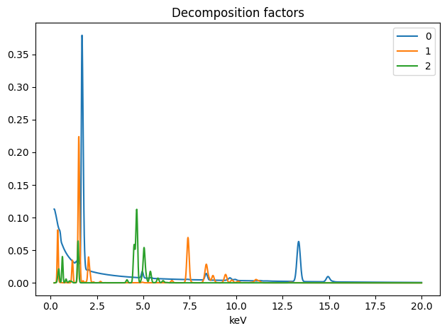
Second cell : Ploting the resulting spectra
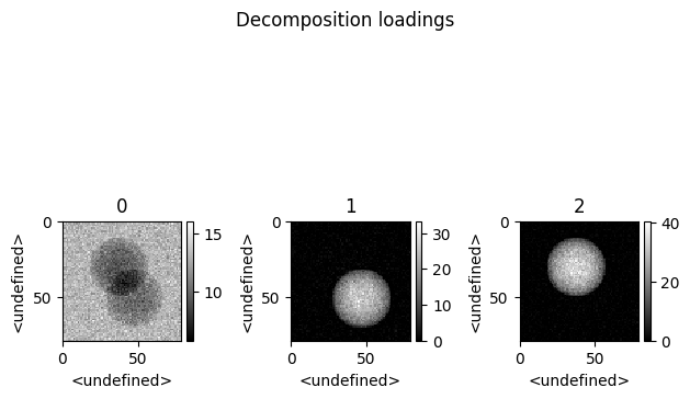
Thrid cell : Ploting the resulting abundances
Hyperspy is mainly designed to be used with the qt graphical backend of matplotlib. Thus two plots will appear if you are in inline mode.
[6]:
spim.print_concentration_report()
+----------+-----------+-------------+-----------+------------+-----------+-------------+
| Elements | p0 (at.%) |  p0 std (%) | p1 (at.%) | p1 std (%) | p2 (at.%) |  p2 std (%) |
+----------+-----------+-------------+-----------+------------+-----------+-------------+
| V        |     4.277 |       0.815 |     0.345 |      5.236 |     0.000 |    5426.344 |
| Rb       |    89.219 |       0.150 |     0.000 |   1217.553 |     0.000 |   10598.007 |
| W        |     6.505 |       0.430 |     0.000 | 329271.319 |     0.000 |      93.434 |
| N        |     0.000 | 3363320.990 |    52.263 |      0.848 |     0.000 |     423.427 |
| Yb       |     0.000 | 1047375.542 |    38.941 |      0.306 |     0.000 | 1344807.923 |
| Pt       |     0.000 | 1056115.743 |     8.450 |      0.663 |     0.000 |     172.133 |
| Al       |     0.000 | 2353678.576 |     0.000 |    307.918 |    23.854 |       0.781 |
| Ti       |     0.000 | 1773459.703 |     0.000 |    447.321 |    23.390 |       0.594 |
| La       |     0.000 | 1510549.003 |     0.000 |  15735.001 |    52.756 |       0.337 |
+----------+-----------+-------------+-----------+------------+-----------+-------------+

Disclaimer : The presented errors correspond to the statistical error on the fitted intensity of the peaks.
In other words it corresponds to the precision of the measurment.
The accuracy of the measurment strongly depends on other factors such as absorption, cross-sections, etc...
Please consider these parameters when interpreting the results.
[7]:
spim.plot_decomposition_loadings(3)
[7]:


[8]:
spim.plot_decomposition_factors(3)
[8]:

