Regularized Poisson NMF on a toy dataset

This notebook is part of the ESPM package. It is available on github

In this notebook, we show how to solve a regularized Poisson Non Negative Matrix Factorization (NMF) on a toy dataset. The general goal of this problem is to separate a matrix \(X\) into two matrices \(D\) and \(H\) such that \(X \approx DH\). We will assume that \(D\) is the product of two matrices \(G\) and \(W\) such that \(D = GW\). The matrix \(G\) is assumed to be known and therefore \(W\) is the matrix we want to find. In the field of electro-microscopy, the matrix \(GW\) represent the phases, the matrix \(H\) is the matrix of maps (or weights) and \(X\) is the data matrix. The maps \(H\) are 2D images. Furthermore, we will assume that \(W, H\) are non-negative or more generally greater than a small positive value \(\epsilon\).

The data measured data \(X\) is follow a Poisson distribution, i.e. \(X_{ij} \sim \text{Poisson}(n_p\dot{X}_{ij})\). In the context of electro-microscopy, \(n_p\) is the number of photons per pixel. \(\dot{X} = G \dot{W} \dot{H}\) would correspond a noiseless measurement.

The size of:

• \(X\) is (n, p),

• \(W\) is (m, k),

• \(H\) is (k, p),

• \(G\) is (n, m).

In general, m is assumed to be much smaller than n and \(G\) is assumed to be known. The parameter shape_2d defines the shape of the images for the columns of \(H\) and \(X\), i.e. shape_2d[0]*shape_2d[1] = p.

Mathematically. the problem can be formulated as:

\[\dot{W}, \dot{H} = \arg\min_{W\geq\epsilon, H\geq\epsilon, \sum_i H_{ij} = 1} D_{GKL}(X || GWH) + \lambda tr ( H^\top \Delta H) + \mu \sum_{i,j} (\log H_{ij} + \epsilon_{reg})\]

Here \(D_{GKL}\) is the fidelity term, i.e. the Generalized KL divergence

\[D_{GKL}(X \| Y) = \sum_{i,j} X_{ij} \log \frac{X_{ij}}{Y_{ij}} - X_{ij} + Y_{ij}\]

The loss is regularized using two terms: a Laplacian regularization on \(H\) and a log regularization on \(H\). \(\lambda\) and \(\mu\) are the regularization parameters. The Laplacian regularization is defined as:

\[\lambda tr ( H^\top \Delta H)\]

where \(\Delta\) is the Laplacian operator (it can be created using the function :mod:espm.utils.create_laplacian_matrix). Note that the columns of the matrices :math:`H` and :math:`X` are assumed to be images.

The log regularization is defined as:

\[\mu \sum_{i,j} (\log H_{ij} + \epsilon_{reg})\]

where \(\epsilon_{reg}\) is the slope of log regularization at 0. This term acts similarly to an L1 penalty but affects less larger values.

Finally, we assume \(W,H\geq \epsilon\) and that the lines of \(H\) sum to 1:

\[\sum_i H_{ij} = 1.\]

This is done by adding the parameter force_simplex=True to the class espm.estimators.SmoothNMF. This constraint is essential as it prevent the algorithm to find a solution where all the maps tend to 0 because of the other constraints.

In this notebook, we will use the class espm.estimators.SmoothNMF to solve the problem.

Imports and function definition

Let’s start by importing the necessary libraries.

# Some useful modules for notebooks
%load_ext autoreload
%autoreload 2
%matplotlib inline

import numpy as np
import matplotlib.pyplot as plt
from espm.estimators import SmoothNMF
from espm.measures import find_min_angle, ordered_mse, ordered_mae, ordered_r2
from espm.models import ToyModel
from espm.weights import generate_weights as gw
from espm.datasets.base import generate_spim_sample
from espm.utils import process_losses

Now we define the parameters that will be used to generate the data.

seed = 42 # for reproducibility

m = 15 # Number of components
n = 200 # Length of the phases

n_poisson = 300 # Average poisson number per pixel (this number will be splitted on the m dimension)

densities = np.random.uniform(0.1, 2.0, 3) # Random densities

def get_toy_sample():
    model_params = {"L": n, "C": m, "K": 3, "seed": seed}
    misc_params = {"N": n_poisson, "seed": seed, 'densities' : densities, "model": "ToyModel"}

    toy_model = ToyModel(**model_params)
    toy_model.generate_phases()
    phases = toy_model.phases.T
    weights = gw.generate_weights("toy_problem", None)

    sample = generate_spim_sample(phases, weights, model_params,misc_params, seed = seed)
    return sample

def to_vec(X):
    n = X.shape[2]
    return X.transpose(2,0,1).reshape(n, -1)

sample = get_toy_sample()

GW = sample["GW"].T
G = sample["G"]
H = to_vec(sample["H"])
X = to_vec(sample["X"])
Xdot = to_vec(sample["Xdot"])
shape_2d = sample["shape_2d"]

Let us look at the dimension of our problem.

print(f"""
- X: {X.shape}
- Xdot: {Xdot.shape}
- G: {G.shape}
- GW: {GW.shape}
- H: {H.shape}
- shape_2d: {shape_2d}
""")

- X: (200, 10000)
- Xdot: (200, 10000)
- G: (200, 15)
- GW: (200, 3)
- H: (3, 10000)
- shape_2d: (100, 100)

Here Xdot contains the noisless data such that the ground truth H and GW satisfies:

\[X = GWH\]

np.testing.assert_allclose(Xdot, GW @ H)

Let us plot the ground truth maps \(H\) (sometimes also called weights). Here the variable shape_2d is used to reshape the columns of \(H\) into images.

vmin, vmax = 0,1
cmap = plt.cm.gray_r
plt.figure(figsize=(10, 3))
for i, hdot in enumerate(H):
    plt.subplot(1,3,i+1)
    plt.imshow(H[i].reshape(shape_2d), cmap=cmap, vmin=vmin, vmax=vmax)
    plt.axis("off")
    plt.title(f"GT - Map {i+1}")

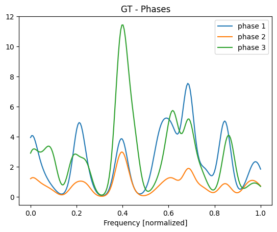
We can also plot the phases corresponding to these maps. The phases corresponds to the matrix \(GW\).

e = np.linspace(0,1, GW.shape[0])
plt.plot(e, GW)
plt.title("GT - Phases")
plt.xlabel("Frequency [normalized]")
plt.legend([f"phase {i+1}" for i in range(3)]);

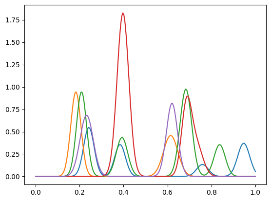
The matrix \(G\) is assumed to be known appriori. Here we plot the first 5 lines of \(G\).

l = np.linspace(0, 1,n)
plt.plot(l, G[:,:5]);

Note that the function create_toy_sample did not return \(W\) but only \(GW\).

Using the ground truth \(GW\), it can be computed as follows:

W = np.linalg.lstsq(GW, G, rcond=None)[0].T
W.shape

(15, 3)

Solving the problem

Parameters

Let us define the different hyperparameters of the problem. Feel free to change them and see how the results change.

Let us first define our regularisation parameters.

lambda_L = 2 # Smoothness of the maps
mu = 0.05 # Sparsity of the maps

We can additionally add a simplex constraint to the problem by setting force_simplex=True. This will add the constraint that the line of \(H\) sum to 1. This constraint should be activated for the regularizers to work!. Practically, it will prevent the algorithm from simply minimizing \(W\) and increasing \(H\).

force_simplex = True

Finally, we can decide to specify \(G\) or not. If the matrix \(G\) is not specified, the algorithm will directly estimate \(GW\) insead of \(W\).

Gused = G

Note that wihtout regularisation, i.e. with the parameters

lambda_L = 0
mu = 0
Gused = None
force_simplex=False

we recover the classical Poisson/KL NMF problem. Our algorithm will apply the MU algorithm from Lee and Seung (2001).

Let us define the parameters for the algorithm. Here the class espm.estimator.SmoothNMF heritates from sckit-learn’s NMF class.

K = len(H) # Number of components / let assume that we know it
params = {}
params["tol"]=1e-6 # Tolerance for the stopping criterion.
params["max_iter"] = 200 # Maximum number of iterations before timing out.
params["hspy_comp"] = False # If should be set to True if hspy data format is used.
params["verbose"] = 1 # Verbosity level.
params["eval_print"] = 10 # Print the evaluation every eval_print iterations.
params["epsilon_reg"] = 1 # Regularization parameter
params["linesearch"] = False # Use linesearch to accelerate convergence
params["shape_2d"] = shape_2d # Shape of the 2D maps
params["n_components"] = K # Number of components
params["normalize"] = True # Normalize the data. It helps to keep the range of the regularization parameters lambda_L and mu in a reasonable range.

estimator = SmoothNMF(mu=mu, lambda_L=lambda_L, G = Gused, force_simplex=force_simplex, **params)

The function fit_transform will solve the problem and return the matrix \(GW\).

GW_est = estimator.fit_transform(X)

It 10 / 200: loss 5.593893e-03,  3.844 it/s
It 20 / 200: loss 5.532716e-03,  3.889 it/s
It 30 / 200: loss 5.509986e-03,  3.904 it/s
It 40 / 200: loss 5.495493e-03,  3.907 it/s
It 50 / 200: loss 5.485530e-03,  3.911 it/s
It 60 / 200: loss 5.477536e-03,  3.917 it/s
It 70 / 200: loss 5.427513e-03,  3.917 it/s
It 80 / 200: loss 5.158176e-03,  3.916 it/s
It 90 / 200: loss 5.098168e-03,  3.904 it/s
It 100 / 200: loss 5.072739e-03,  3.893 it/s
It 110 / 200: loss 5.054121e-03,  3.891 it/s
It 120 / 200: loss 5.039331e-03,  3.894 it/s
It 130 / 200: loss 5.026454e-03,  3.895 it/s
It 140 / 200: loss 5.015486e-03,  3.897 it/s
It 150 / 200: loss 5.006813e-03,  3.899 it/s
It 160 / 200: loss 5.000377e-03,  3.901 it/s
It 170 / 200: loss 4.995725e-03,  3.902 it/s
It 180 / 200: loss 4.992326e-03,  3.904 it/s
It 190 / 200: loss 4.989736e-03,  3.905 it/s
exits because max_iteration was reached
Stopped after 200 iterations in 0.0 minutes and 51.0 seconds.

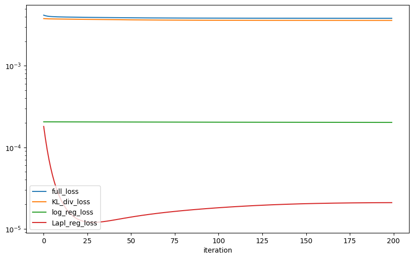
We can plot the different losses to see how the algorithm converges.

losses = estimator.get_losses()

values, names = process_losses(losses)

plt.figure(figsize=(10, 6))
for name, value in zip(names[:4], values[:4]):
    plt.plot(value, label=name)
    plt.xlabel("iteration")
plt.yscale("log")
plt.legend()

<matplotlib.legend.Legend at 0x7fef18ee7ed0>

losses[0]

(0.00597679, 0.00558329, 0.00020724, 0.00018625, 8., 0.72441301, 0.79218163)

We can easily recover \(W\) and \(H\) from the estimator.

H_est = estimator.H_
W_est = estimator.W_

Let us compute some metrics to evaluate the quality of the solution. We will use the metrics defined in the module espm.metrics.

We first compute the angles between the phases GW and the estimated phases GW_est. The angles are computed using the function compute_angles. This function also return the indices to match the estimations and the ground truths. Indeed, there is no reason for them to have the same order.

angles, true_inds = find_min_angle(GW.T, GW_est.T, unique=True, get_ind=True)
print("angles : ", angles)

angles :  [7.344652590769181, 13.301110152431441, 34.07026785204474]

Now, we can compute the Mean Squared Error (MSE) between the maps H and the estimated maps H_est.

mse = ordered_mse(H, H_est, true_inds)
print("mse : ", mse)

mse :  [0.03782827121738191, 0.009546793204048424, 0.020481964919775702]

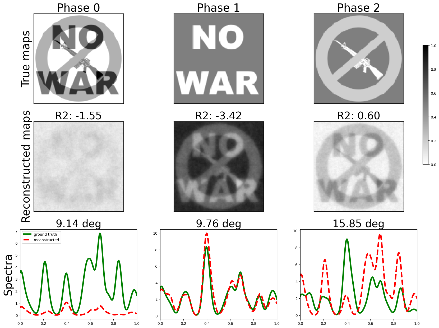
Finally, let us plot the results.

def plot_results(Ddot, D, Hdotflat, Hflat):
    fontsize = 30
    scale = 15
    aspect_ratio = 1.4
    marker_list = ["-o","-s","->","-<","-^","-v","-d"]
    mark_space = 20
    # cmap = plt.cm.hot_r
    cmap = plt.cm.gray_r
    vmax = 1
    vmin = 0
    K = len(H)
    L = len(D)

    angles, true_inds = find_min_angle(Ddot.T, D.T, unique=True, get_ind=True)
    mse = ordered_mse(Hdotflat, Hflat, true_inds)
    mae = ordered_mae(Hdotflat, Hflat, true_inds)
    r2 = ordered_r2(Hdotflat, Hflat, true_inds)


    fig, axes = plt.subplots(K,3,figsize = (scale/K * 3 * aspect_ratio,scale))
    x = np.linspace(0,1, num = L)
    for i in range(K):
        axes[2,i].plot(x,Ddot.T[i,:],'g-',label='ground truth',linewidth=4)
        axes[2,i].plot(x,D[:,true_inds[i]],'r--',label='reconstructed',linewidth=4)
        axes[2,i].set_title("{:.2f} deg".format(angles[i]),fontsize = fontsize-2)
        axes[2,i].set_xlim(0,1)

        axes[1,i].imshow((Hflat[true_inds[i],:]).reshape(shape_2d),vmin = vmin, vmax = vmax , cmap=cmap)
        axes[1,i].set_title("R2: {:.2f}".format(r2[true_inds[i]]),fontsize = fontsize-2)
        # axes[i,1].set_ylim(0.0,1.0)
        axes[1,i].tick_params(axis = "both",labelleft = False, labelbottom = False,left = False, bottom = False)

        im = axes[0,i].imshow(Hdotflat[i].reshape(shape_2d),vmin = vmin, vmax = vmax, cmap=cmap)
        axes[0,i].set_title("Phase {}".format(i),fontsize = fontsize)
        axes[0,i].tick_params(axis = "both",labelleft = False, labelbottom = False,left = False, bottom = False)
        axes[2,0].legend()

    rows = ["True maps","Reconstructed maps","Spectra"]

    for ax, row in zip(axes[:,0], rows):
        ax.set_ylabel(row, rotation=90, fontsize=fontsize)


    fig.subplots_adjust(right=0.84)
    # put colorbar at desire position
    cbar_ax = fig.add_axes([0.85, 0.5, 0.01, 0.3])
    fig.colorbar(im,cax=cbar_ax)

    # fig.tight_layout()

    print("angles : ", angles)
    print("mse : ", mse)
    print("mae : ", mae)
    print("r2 : ", r2)

    return fig

fig = plot_results(GW, GW_est, H, H_est)
plt.show()

angles :  [7.344652590769181, 13.301110152431441, 34.07026785204474]
mse :  [0.03782827121738191, 0.009546793204048424, 0.020481964919775702]
mae :  [0.1837367734355168, 0.07608034822853892, 0.129948436009346]
r2 :  [0.48546361971274876, 0.6065982205085647, 0.5272447963807385]