Models

The espm.models module implements the model objects that are used to simulate features of the data (e.g. in EDXS it corresponds to spectra). The models are also used for the creation of the G matrix, which can be later used for the decomposition of data using NMF.

Note

For now espm supports only the modelling of EDS data but we aim at supporting the modelling of EELS data too.

Models base classes

The PhysicalModel is the abstract class from which the EDX model inherits. The ToyModel can be used for testing data analysis algorithms.

class espm.models.base.Model

Abstract class for models.

abstract generate_g_matr(g_parameters)

abstract generate_phases(phase_parameters)

class espm.models.base.PhysicalModel(e_offset, e_size, e_scale, params_dict, db_name='default_xrays.json', E0=200, **kwargs)

Abstract class of the models

build_energy_scale(e_offset, e_size, e_scale)

Build an array corresponding to a linear energy scale.

Parameters:

e_offset

float:

Offset of the energy scale

e_size

int:

Number of channels of the detector

e_scale

float:

Scale in keV/channel

Returns:

energy scale

np.array 1D:

Linear energy scale based on the given parameters of shape (e_size,)

extract_DB(db_name)

Read the cross-sections from the database

Parameters:

db_name

string:

Name of the json database file

Returns:

data

dict:

A dictionnary containing the cross-sections in the database

extract_DB_mdata(db_name)

Read the metadata of the database

Parameters:

db_name

string:

Name of the json database file

Returns:

data

dict:

A dictionnary containing the metadata related to the database

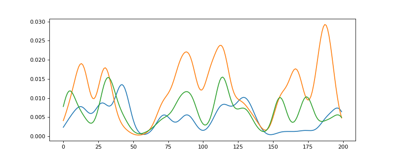
class espm.models.base.ToyModel(L: int = 200, C: int = 15, K: int = 3, seed: int | None = None)

Toy model.

Simple model with a random G matrix and phases.

The G matrix is generated with a random number of gaussians per column. The phases are generated using a vector drawn from a Laplacian distribution and multiplied by the G matrix.

Parameters:

Lint

Length of the phases.

Cint

Number of possible components in the phases.

Kint

Number of phases.

seedint, optional

Seed for the random number generator.

Examples

>>> from espm.models import ToyModel
>>> import matplotlib.pyplot as plt
>>> model = ToyModel(L=200, C=15, K=3, seed=0)
>>> model.generate_g_matr()
>>> model.generate_phases()
>>> print(model.G.shape)
(200, 15)
>>> print(model.phases.shape)
(200, 3)
>>> plt.plot(model.phases)

generate_g_matr(*args, **kwargs) → None

Generate G matrix.

Parameters:

argsignored

kwargsignored

Returns:

None

generate_phases(*args, **kwargs) → None

Generate phases.

Parameters:

argsignored

kwargsignored

Returns:

None

EDXS model

The espm.models.edxs module implements the creation of the G matrix that contains a modelisation of the characteristic and continuous X-rays.

This module is a key component of the EDXS data simulation and the EDXS data analysis.

class espm.models.edxs.EDXS(*args, width_slope=0.01, width_intercept=0.065, **kwargs)

generate_g_matr(g_type='bremsstrahlung', reference_elt={}, stoichiometries=[], *, elements=[], **kwargs)

Generate the G matrix. With a complete model the matrix is (e_size,n+2). The first n columns correspond to the sum of X-ray characteristic peaks associated to each shell of the elements. The last 2 columns correspond to a bremsstrahlung model.

The first n columns of G (noted \(\kappa\)), corresponding to the characteristic X-rays, can be calculated using the following formula:

\[\kappa_{k,Z} = \sum_{ij} x_{ij}(Z) \frac{1}{\Delta(\varepsilon_k) \sqrt{2\pi} } e{^{-\frac{1}{2} {\left( \frac{\varepsilon_k - \varepsilon^{ij}(Z)}{\Delta(\varepsilon_k)} \right)}^2}}\]

where \(\varepsilon_k\) is the energy of the kth energy channel, \(\varepsilon^{ij}(Z)\) is the energy of the ijth line of the Zth element, \(\Delta(\varepsilon_k)\) is the FWHM of the detector at the energy \(\varepsilon_k\) and \(x_{ij}(Z)\) is the intensity ratio of the ijth line of the Zth element. The last term of the equation is a gaussian function centered at \(\varepsilon^{ij}(Z)\) and with a FWHM of \(\Delta(\varepsilon_k)\).

The last two columns of G (noted \(\beta\)), corresponding to the bremsstrahlung model, can be calculated using the following formula:

\[ \begin{align}\begin{aligned}\beta_{k,n+1} = \frac{\varepsilon_0 - \varepsilon_k}{\varepsilon_0 \varepsilon_k} \times \frac{1 - (\varepsilon_0 - \varepsilon_k)}{\varepsilon_0}\\\beta_{k,n+2} = \frac{(\varepsilon_0 - \varepsilon_k)^2}{\varepsilon^2_0 \varepsilon_k}\end{aligned}\end{align} \]

Note that there is no parameter for the bremsstrahlung since it is supposed to be learned with the W matrix (see espm.estimators).

Parameters:

g_type

string:

Options of the edxs model to include in the G matrix. The three possibilities are “identity”, “no_brstlg” and “bremsstrahlung”. G is going to be the identity matrix, only characteristic X-ray peaks or characteristic X-rays plus bremsstrahlung model, respectively.

reference_elt

dict:

The keys are chemical elements (atomic number) and the values are cut-off energies. This argument is used to split some of the columns of G into 2 columns. The first column corresponds to characteristic X-rays before the cut-off and second one corresponds to characteristic X-rays before the cut-off. This feature is implemented to enable more accurate absorption correction.

elements

list:

List of modeled chemical elements. The list can be populated either with atomic numbers or chemical symbols, e.g. “Fe” or 26.

stoichiometries

list:

Optional list of stoichiometries as strings. Each string represent a fixed stoichiometry such as “Fe3O4” and calculate an addtional column of G for it to help the decomposition.

Returns:

g matrix

np.array 2D:

matrix of the edx model.

Notes

See our paper about the espm package [TPH+23] for more information about the equations of this model.

generate_phases(phases_parameters)

Generate a series of spectra from list of phase parameters.

Parameters:

phases_parameters

list:

List of dicts containing the phase parameters.

Returns:

phase_array

np.array 2D:

Array which lines correspond to the modelled phases in the input list.

Notes

The absorption correction is done using the average composition of the phases. The same correction is used for each phase.

generate_spectrum(b0=0, b1=0, scale=1.0, abs_elts_dict={}, *, elements_dict={})

Generate a spectrum from bremsstrahlung parameters and a chemical composition. The modelling is done using the same formula as for the generate_g_matr function.

Parameters:

b0

float:

First bremsstrahlung parameter.

b1

float:

Second bremsstrahlung parameter.

scale

float:

Scale factor to apply to the bremsstrahlung. Feature to be removed, scaling should be done with b0 and b1.

abs_elts_dict

dict:

Dictionnary of elements and associated concentrations. This dictionnary is used to calculate the contribution of the absorption in the spectrum.

elements_dict

dict:

Dictionnary of elements and associated concentrations describing the chemical composition of the modeled sample.

Returns

——-

spectrum

np.array 1D:

Output edx spectrum corresponding to the input chemical composition.

Notes

Check EDXS_function for details about the bremsstrahlung model.

Examples

>>> import matplotlib.pyplot as plt
>>> from espm.models.edxs import EDXS
>>> from espm.conf import DEFAULT_EDXS_PARAMS
>>> b0, b1 = 5.5367e-5, 0.00192181
>>> elts_dict = {"Si" : 1.0,"Ca" : 1.0,"O" : 3.0,"C" : 0.3}
>>> model = EDXS(**DEFAULT_EDXS_PARAMS)
>>> spectrum = model.generate_spectrum(b0,b1, elements_dict = elts_dict)
>>> plt.plot(spectrum)

espm.models.edxs.G_EDXS(model, g_params, part_W=None, G=None)

Update the bremsstrahlung part of the G matrix. This function is used for the NMF decomposition so that the absorption correction is updated in between each step.

Parameters:

model_params

dict:

Parameters of the edxs model. Check espm.conf.DEFAULT_EDXS_PARAMS for an example.

g_params

dict:

Parameters specific to the creation of the G matrix.

part_W

np.array 2D:

Concentrations determined during the NMF decomposition. It is used to determine the average composition that will be used to determine the absorption correction.

G

np.array 2D:

Current G matrix. Setting it to None will initialize the G matrix.

Returns:

updated G

np.array 2D:

Updated G matrix with a new absorption correction.

EDXS functions

The espm.models.EDXS_function module implements misceallenous functions required for the :mod: espm.models.edxs. This module include bremsstrahlung modelling, database reading and dicts and list manipulation functions.

espm.models.EDXS_function.G_bremsstrahlung(x, E0, params_dict, *, elements_dict={})

Computes the two-parts continuum X-rays for the G matrix. The two parts of the bremsstrahlung are constructed separately so that its parameters can fitted to data. Absorption and detection are multiplied to each part.

Parameters:

x

np.array 1D:

Energy scale.

params_dict

dict:

Dictionnary containing the absorption and detection parameters.

elements_dict

dict:

Composition of the studied sample. It is required for absorption calculation.

Returns:

continuum_xrays

np.array 2D:

Two parts continuum X-rays model with shape (energy scale size, 2).

espm.models.EDXS_function.chapman_bremsstrahlung(x, b0, b1, b2)

Calculate the bremsstrahlung as parametrized by chapman et al.

Parameters:

x

np.array 1D:

Energy scale.

b0

float:

First parameter, corresponding to the inverse of the energy.

b1

float:

Second parameter, corresponding to the energy.

b2

float:

Third parameter, corresponding to the square of the energy.

Returns:

bremsstrahlung

np.array 1D:

Bremsstrahlung model

Notes

For details see [CNC84]

espm.models.EDXS_function.continuum_xrays(x, params_dict={}, b0=0, b1=0, E0=200, *, elements_dict={'Si': 1.0})

Computes the continuum X-rays, i.e. the bremsstrahlung multiplied by the absorption and the detection efficiency.

Parameters:

x

np.array 1D:

Energy scale.

params_dict

dict:

Dictionnary containing the absorption and detection parameters.

b0

float:

First parameter.

b1

float:

Second parameter.

E0

float:

Energy of the incident beam in keV.

elements_dict

dict:

Composition of the studied sample. It is required for absorption calculation.

Returns:

continuum_xrays

np.array 1D:

Continuum X-rays model.

Notes

• When an empty dict is provided. The continuum X-rays are set to 0. This is useful to perform calculations without the bremsstrahlung for example.

• For an example structure of the params_dict parameter, check the DEFAULT_EDXS_PARAMS espm.conf.

• For a custom detection efficiency, check the spectrum fit notebook.

espm.models.EDXS_function.elts_dict_from_W(part_W, *, elements=[])

Create a dictionnary of the elemental concentration from a fitted W. It useful to recompute absorption during the our custom NMF calculations.

Parameters:

part_W

np.array 2D:

W matrix output from the NMF calculation. It only makes sense when the NMF decomposition if performed with G.

elements

list:

List of elements as atomic number or symbol.

Returns:

elements_dictionnary

dict:

Dictionnary containing the concentration associated to each chemical element of the problem.

Notes

This function should maybe move to another part of espm.

Examples

>>> import numpy as np
>>> from espm.models.EDXS_function import elts_dict_from_W
>>> W = np.ones((4,3))
>>> elts = ["Si","Ca","O","C"]
>>> elts_dict_from_W(W,elements = elts)
    {"Si" : 0.25, "Ca" : 0.25, "O" : 0.25, "C" : 0.25}

espm.models.EDXS_function.elts_dict_from_dict_list(dict_list)

Create a single dictionnary of the elemental concentration from a list of dictionnary containing chemical compositions. The new dictionnary corresponds to the average chemical composition of the list.

Parameters:

dict_list

list [dict]:

list of chemical composition dictionnary

Returns:

elements_dictionnary

dict:

Dictionnary containing the concentration associated to each chemical elements contained in the input.

Notes

This function should maybe move to another part of espm.

Examples

>>> import numpy as np
>>> from espm.models.EDXS_function import elts_dict_from_dict_list
>>> dicts = [{"Si" : 1.0},{"Ca" : 1.0},{"O" : 1.0},{"C" : 1.0}]
>>> elts_dict_from_dict_list(dicts)
    {"Si" : 0.25, "Ca" : 0.25, "O" : 0.25, "C" : 0.25}

espm.models.EDXS_function.elts_list_from_dict_list(dict_list)

Create a list of elements from a list of dictionnary containing chemical compositions. The list contains all the elements contained in the input.

Parameters:

dict_list

list [dict]:

list of chemical composition dictionnary

Returns:

elements_list

list:

List of elements as atomic number or symbol.

Examples

>>> import numpy as np
>>> from espm.models.EDXS_function import elts_list_from_dict_list
>>> dicts = [{"Si" : 1.0, "C" : 0.5, "O" : 0.5},{"Ca" : 1.0, "K" : 2.0},{"O" : 1.0, "Si" : 0.5},{"C" : 1.0}] 
>>> elts_list_from_dict_list(dicts)
    ["Si","Ca","O","C","K"]

espm.models.EDXS_function.gaussian(x, mu, sigma)

Calculate the gaussian function according to the following formula:

\[f(x) = \frac{1}{\sigma \sqrt{2 \pi}} e^{-\frac{(x-\mu)^2}{2 \sigma^2}}\]

Parameters:

xnp.array 1D

Energy scale.

mufloat

Mean of the gaussian.

sigmafloat

Standard deviation of the gaussian.

Returns:

gaussiannp.array 1D

Gaussian distribution on x, with mean mu and standard deviation sigma.

espm.models.EDXS_function.lifshin_bremsstrahlung(x, b0, b1, E0=200)

Calculate the custom parametrized bremsstrahlung inspired by the model of L.Lifshin.

The model is designed to have the same definition set as the original model of L.Lifshin with \(b_0 > 0\) and \(b_1 > 0\).

The model is defined as follows:

\[f(\varepsilon) = b_0 \frac{\varepsilon_0 - \varepsilon}{\varepsilon_0 \varepsilon} \left(1 - \frac{\varepsilon_0 - \varepsilon}{\varepsilon_0}\right) + b_1 \frac{\left( \varepsilon_0 - \varepsilon \right) ^2}{\varepsilon_0^2 \varepsilon}\]

where \(\varepsilon_0\) is the energy of the incident beam, \(\varepsilon\) is the energy of the emitted photon and \(b_0\) and \(b_1\) are the parameters of the model.

Parameters:

x

np.array 1D:

Energy scale.

b0

float:

First parameter.

b1

float:

Second parameter.

E0

float:

Energy of the incident beam in keV.

Returns:

bremsstrahlung

np.array 1D:

Bremsstrahlung model

Notes

For details see L.Lifshin, Ottawa, Proc.9.Ann.Conf.Microbeam Analysis Soc. 53. (1974)

espm.models.EDXS_function.lifshin_bremsstrahlung_b0(x, b0, E0=200)

Calculate the first part of our bremsstrahlung model.

espm.models.EDXS_function.lifshin_bremsstrahlung_b1(x, b1, E0=200)

Calculate the second part of our bremsstrahlung model.

espm.models.EDXS_function.read_compact_db(elt, db_dict)

Read the energy and cross section of each line of a chemical element for compact databases.

Parameters:

elt

string:

Atomic number.

db_dict

dict:

Dictionnary extracted from the json database containing the emission lines and their energies.

Returns:

energies

list float:

List of energies associated to each emission line of the given element

cross-sections

list float:

List of emission cross-sections of each line of the given element

espm.models.EDXS_function.read_lines_db(elt, db_dict)

Read the energy and cross section of each line of a chemical element for explicit databases.

Parameters:

elt

string:

Atomic number.

db_dict

dict:

Dictionnary extracted from the json database containing the emission lines and their energies.

Returns:

energies

list float:

List of energies associated to each emission line of the given element

cross-sections

list float:

List of emission cross-sections of each line of the given element

espm.models.EDXS_function.shelf(x, height, length)

Calculate the shelf contribution of the EDXS Silicon Drift Detector (SDD) detector.

Parameters:

x

np.array 1D:

Energy scale.

height

float:

Height in intensity of shelf contribution of the detector.

length

float:

Length in energy of shelf contribution of the detector.

Returns:

shelf

np.array 1D:

SDD shelf model.

Notes

For details see [SP09]

espm.models.EDXS_function.update_bremsstrahlung(G, part_W, model, elements_list)

Update the continuum X-rays part of the G matrix with the current average chemical composition.

Parameters:

G

np.array 2D:

EDXS modelling matrix.

part_W

np.array 2D:

Learned chemical concentrations.

model

espm.models.EDXS:

EDXS model.

elements_list

list:

List of elements as atomic number or symbol.

Returns:

new_G

np.array 2D:

New G matrix with updated continuum X-rays models.

Notes

This function should maybe move to another part of espm.

Absorption functions

The espm.models.absorption_edxs module implements the functions to calculate the contribution of absorption in edx spectra.

espm.models.absorption_edxs.absorption_coefficient(x, atomic_fraction=False, *, elements_dict={'Si': 1.0})

Calculate the mass-absorption coefficent of a given composition at a certain energy or over a certain energy range.

Parameters:

x

np.array 1D:

Energy value or energy scale over which the mass-absorption coefficient is calculated.

atomic_fraction

boolean:

If True, the atomic concentrations of elements_dict are converted in atomic weight fractions.

elements_dict

dict:

Dictionnary with chemical elements as keys and atomic weight fractions (or atomic concentrations) as values.

Returns:

mass-absorption coefficient

np.array 1D:

Calculated value of the mass-absorption coefficient on all the energy range.

Notes

The mass-absorption coefficients are calculated using the database of hyperspy [dlPPF+22].

espm.models.absorption_edxs.absorption_correction(x, thickness=1e-05, toa=90, density=None, atomic_fraction=False, *, elements_dict={'Si': 1.0}, **kwargs)

Calculate the contribution of the absorption on the EDX spectrum for a thin slab of material with a given composition at a certain energy or over a certain energy range. The absorption correction is calculated using the following formula :

\[\frac{1 - \exp(-\chi)}{\chi} \]

where \(\chi = \mu \rho t / \sin(\theta)\), \(\mu\) is the mass-absorption coefficient, \(\rho\) is the density of the material, \(t\) is the thickness of the sample and \(\theta\) is the average take-off angle of the x-rays travelling from the sample to the x-ray detectors.

Parameters:

x

np.array 1D:

Energy value or energy scale over which the mass-absorption coefficient is calculated.

thickness

float:

Thickness of the material slab in meter. If the thickness is set to 0.0, the function will return 1.0.

toa

float:

Take-off angle in degrees of the x-rays travelling from the sample to the x-ray detectors.

density

float:

Density of the material in g/m3 (to be checked). If None, an approximation of the density based on the atomic numbers of the elements of the materials is calculated.

atomic_fraction

boolean:

If True, the atomic concentrations of elements_dict are converted in atomic weight fractions.

elements_dict

dict:

Dictionnary with chemical elements as keys and atomic weight fractions (or atomic concentrations) as values.

Returns:

absorption correction

np.array 1D:

Calculated value of the absorption correction on all the energy range.

espm.models.absorption_edxs.absorption_mass_thickness(x, mass_thickness, toa=90, atomic_fraction=True, *, elements_dict={'Si': 1.0})

Calculate the contribution of the absorption of a mass-thickness map.

Parameters:

x

np.array 1D:

Energy value or energy scale over which the mass-absorption coefficient is calculated.

mass_thickness:

np.array 2D:

Mass-thickness map. See the notes for details.

toa

float:

Take-off angle in degrees of the x-rays travelling from the sample to the x-ray detectors.

atomic_fraction

boolean:

If True, the atomic concentrations of elements_dict are converted in atomic weight fractions.

elements_dict

dict:

Dictionnary with chemical elements as keys and atomic weight fractions (or atomic concentrations) as values.

Returns:

absorption correction

np.array 3D:

Calculated value of the absorption correction on all the energy range for all pixels of the mass-thickness map.

Notes

The mass-thickness map can be extracted from an EDX spectrum image by calculating the concentration of an element for both K and L lines. Since there should be only one concentration for both lines, it is possible to determine the contribution of the absorption for each pixel and thus obtain the mass-thickness map.

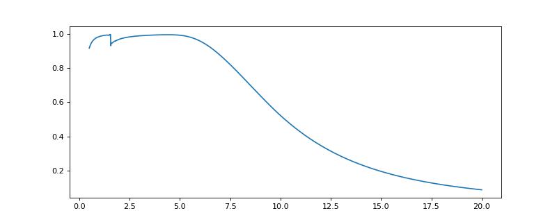
espm.models.absorption_edxs.det_efficiency(x, det_dict)

Simulate the detection efficiency of an EDX detector. The absorption wihtin one layer of the detector is calculated according to the following equation, corresponding to the Beer-Lambert law:

\[d_k = \exp\left( - \mu(\varepsilon_k)\rho t \right)\]

where \(d_k\) is the detection efficiency at the energy \(\varepsilon_k\), \(\mu(\varepsilon_k)\) is the mass-absorption coefficient at the energy \(\varepsilon_k\), \(\rho\) is the density of the material, and \(t\) is the thickness of the material.

In a detection layer of the detector, an absobed photon counts as a detected photon so that the detection efficiency is equal to 1 minus the absorption. The detection efficiency is calculated as the product of the absorption of each layer of the detector.

Parameters:

x

np.array 1D:

Energy value or energy scale over which the mass-absorption coefficient is calculated.

det_dict

dict:

See Examples for an example of the structure of the dict. One of the layer of the input dictionnary should be named “detection” to model a active layer of the detector.

Returns:

efficiency

np.array 1D:

Calculated detection efficiency based on the input layers model.

Examples

>>> from espm.models.absorption_edxs import det_efficiency
>>> import matplotlib.pyplot as plt
>>> import numpy as np
>>> dict = {"detection" : {"thickness" : 10e-3, "density" : 2.3, "atomic_fraction" : False, "elements_dict" : {"Si" : 1.0}},
>>> "dead_layer" : {"thickness" : 50e-7, "density" : 2.7, "atomic_fraction" : False, "elements_dict" : {"Al" : 1.0}}}
>>> x = np.linspace(0.5,20,num = 1000)
>>> efficiency = det_efficiency(x,dict)
>>> plt.plot(x,efficiency)

espm.models.absorption_edxs.det_efficiency_from_curve(x, filename, kind='cubic')

Interpolate a detection efficiency curve that is stored in ~/espm/tables.

Parameters:

x

np.array 1D:

Energy value or energy scale over which the mass-absorption coefficient is calculated.

filename:

string:

Name of the file of the detection efficiency.

kind

string:

Polynomial order of the interpolation.

Returns:

Detection efficiency

np.array 1D:

Interpolated detection efficiency.

espm.models.absorption_edxs.det_efficiency_layer(x, thickness=1e-05, density=None, atomic_fraction=False, *, elements_dict={'Si': 1.0})

Calculate the proportion of absorbed X-rays for one virtual layer of the detector.

Parameters:

x

np.array 1D:

Energy value or energy scale over which the mass-absorption coefficient is calculated.

thickness

float:

Thickness of the material slab in meter. If the thickness is set to 0.0, the function will return 1.0.

density

float:

Density of the material in g/m3 (to be checked). If None, an approximation of the density based on the atomic numbers of the elements of the materials is calculated.

atomic_fraction

boolean:

If True, the atomic concentrations of elements_dict are converted in atomic weight fractions.

elements_dict

dict:

Dictionnary with chemical elements as keys and atomic weight fractions (or atomic concentrations) as values.

Returns:

absorption

np.array 1D:

Calculated absorption of one layer of the detector.

Notes

We assume that the X-rays arrive perpendicular to the detector.

espm.models.generate_EDXS_phases.generate_brem_params(seed)

Generate random parameters for the Bremsstrahlung model with a scaling factor that somewhat resembles the real data.

Parameters:

seedint

Seed for the random number generator.

Returns:

dict

Dictionary containing the parameters for the Bremsstrahlung model.

espm.models.generate_EDXS_phases.generate_elts_dict(seed, nb_elements=3)

Generate a random dictionary of elements and their relative abundance. The elements are limited to the range 6-82.

Parameters:

seedint

Seed for the random number generator.

nb_elementsint, optional

Number of elements to generate. The default is 3.

Returns:

dict

Dictionary containing the elements and their relative abundance.

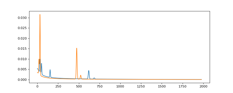
espm.models.generate_EDXS_phases.generate_modular_phases(elts_dicts=3, brstlg_pars=None, scales=None, model_params=None, seed=0)

Generate an array of phases of the EDXS model with set model parameters, elemental compositions and bremsstrahlung parameters.

Parameters:

elts_dictsint or list, optional

Number of phases to generate or list of dictionnaries containing the chemical compositions. The default is 3.

brstlg_parslist, optional

List of dictionnaries containing the bremsstrahlung parameters. If the parameters are not set, they are generated randomly.

scaleslist, optional

List of scaling factors for the phases. If the scales are not set, they are set to 1.0.

model_paramsdict, optional

Dictionary containing the model parameters. If the parameters are not set, they are set to the default values. See the config file for the default values.

seedint, optional

Seed for the random number generator. The default is 0.

Returns:

np.array

Array of phases of the EDXS model.

Examples

>>> from espm.models.generate_EDXS_phases import generate_modular_phases
>>> import matplotlib.pyplot as plt
>>> phases = generate_modular_phases(elts_dicts = [{"8": 0.5, "14": 0.2, "26": 0.3}, {"8" : 0.5, "23" : 0.3, "7" : 0.2}],
... brstlg_pars = [{"b0" : 0.03, "b1" : 0.01}, {"b0" : 0.002, "b1" : 0.0025}])
>>> plt.plot(phases[0])
>>> plt.plot(phases[1])

espm.models.generate_EDXS_phases.generate_random_phases(n_phases=3, seed=0)

Generate a list of phases of the EDXS model with random elemental compositions and Bremsstrahlung parameters. The model parameters are set to the default values.

Parameters:

n_phasesint, optional

Number of phases to generate. The default is 3.

seedint, optional

Seed for the random number generator. The default is 0.

Returns:

np.array

Array of phases of the EDXS model.

espm.models.generate_EDXS_phases.unique_elts(dict_list)

Generate a list of unique chemical elements from a list of chemical elements dictionnaries.

Parameters:

dict_listlist

List of dictionnaries containing the elements and their relative abundance.

Returns:

list

List of unique chemical elements.

Examples

>>> unique_elts([{"elements_dict" : {"18" : 0.2, "8" : 0.5, "12" : 0.3}}, {"elements_dict" : {"8" : 0.5, "26" : 0.3, "14" : 0.2}}])
['18', '8', '12', '26', '14']